Following a Structure When Performance Tuning, Part 1

So, you have a database or block of code. You’ve been told to “make it fast” but you’re not sure where to start. I’ve got you. We’re going to create a process to follow to ensure we can tune effectively and prove that we’ve made things faster. It’s all about having a structure when performance tuning.

Identification

The first thing is finding those problem queries. You may have the procedure that’s causing problems and we’ll get to the process of tuning later in the article. But let’s assume that we need to find problem queries ourselves.

There’s a couple of different things we can do here depending on the tools you have available. If you have a database monitoring tool in your environment, then you can totally use the functionality in there. I’m going to assume that we’re just using native features of SQL Server, as everybody has access to these.

Query Store

This feature was introduced in SQL Server 2016 and is baked into the engine. It is optional and the default is to have this disabled. See our blog and webinar here for more information. In summary we recommend you turn this on by default in all environments, and only turn it off if you have a good reason to do so.

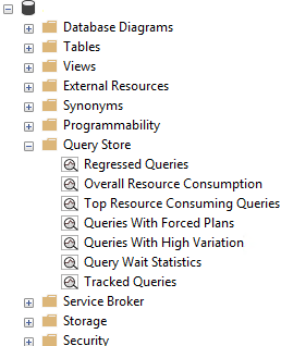
You have a number of reports available within the query store. Have a look through them and get comfortable but the one we’re going to start with, for the purpose of highlighting problem queries, is the Top Resource Consuming Queries report.

Use the Configuration button in the top right corner. The default report shows 30 minutes worth of data, you’ll want to push that out to a week or a month to find your real problem queries.

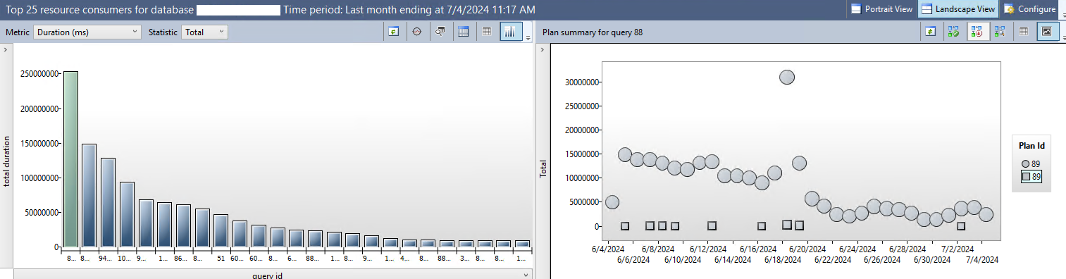
The column graph in the example above shows the total duration for all executions of the query. The graph can be changed to show different metrics (e.g. Duration, CPU, Reads, Memory Consumers) as well as different statistics (e.g. Total, Avg, Max, Min). Have a play and decide which of these queries you want to focus on. If your environment runs hot on CPU, then you may want to focus there first.

The graph on the right shows all plans associated with the query along with any failures (the squares). By hovering over each dot you can see further metrics that are very interesting for nerds like us.

Sp_BlitzCache

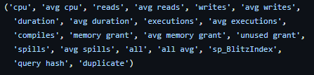
This is an open source stored procedure that’s great for digging into the query plan cache. We can use a number of parameters here; the most common one is @sort_order. This allows you to pass through a number of values to get the most expensive queries in each of these categories.

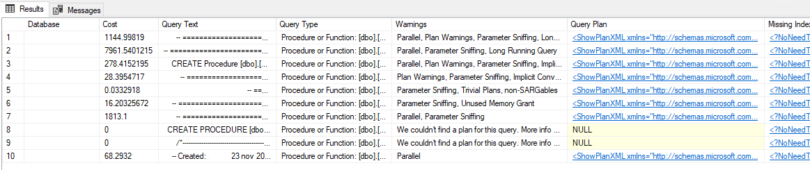
Whatever you choose to sort by, you’ll get a sorted list of queries, the databases they live in, and a lot of very useful information. It will even give you warnings on potential issues with each of the queries that you can use to focus down on the issues.

You can find sp_BlitzCache as part of the First Responder Kit on GitHub here.

Baseline

Before we can make things better with the queries we’ve identified, we need to know how bad they currently are. Ultimately, we’re going to need to make a version of our code that is runnable for testing purposes. I do heavily suggest using a testing environment for performance testing so that you don’t impact your production environment. Make your dev environment as close as possible to production. We’re talking similar hardware specs and similar data size (ideally you can copy the prod database to dev) to ensure we’re comparing apples to apples when tuning our query.

Once you’ve got your environment ready, make the query runnable. If you’re lucky, we’re just running a select query and we have no issues.

In other scenarios, the code may include DML statements (inserts, updates, deletes) into permanent tables (not just temp tables). For these, it’s usually reasonable to wrap your entire block of code in a BEGIN TRANSACTION…. ROLLBACK TRANSACTION. This isn’t perfect and is scary in production environments as your INT values will still increment in tables with IDENTITY columns and you may have gaps in your ID fields. In development environments this is much less of an issue.

You’ll also have to declare any variables that the code may use. Hopefully you’ll already have these captured. However, if you don’t, you have a couple of options. You could speak to any team members who are complaining about the performance and see what parameters they use. If you don’t have this, then I’ve found the best way is to look at the fields that we’re comparing to, find the most common value, and go with this.

Once it’s able to run, we’re going to gather two sets of metrics: the Actual Query Plan and the query statistics.

The Actual Query Plan is simple to enable. Just click this button (circled in red in the image blow) at the top of SSMS. The next time you run the query, it will gather the actual plan in its own tab next to the results and messages tabs.

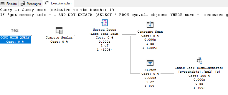
Save the .sqlplan file here for comparison purposes later.

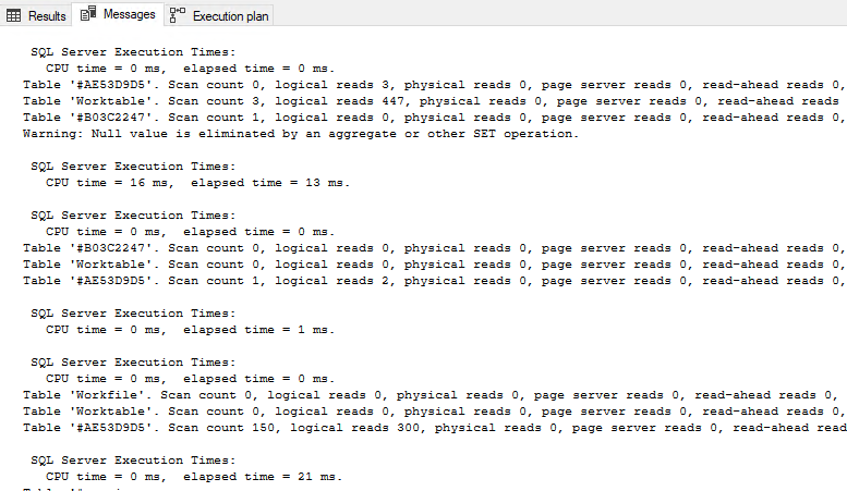
To enable the gathering of statistics, add one simple line of code to the top of your query:;

Source code

SET STATISTICS TIME,IO ON

This will enable the capture of the Time and IO statistics collection. Once you do this and run your query you will have the statistics output into the Messages tab in SSMS.

This is not easy for a human to read and gets complicated with multiple statements within the same query. To make this simple to read, copy the output of the messages tab (ctrl+a, ctrl+V) and paste into statisticsparser.com. Once you click parse, scroll to the bottom of the page and check the summary table. It will have some very valuable information that we’ll use as the baseline.

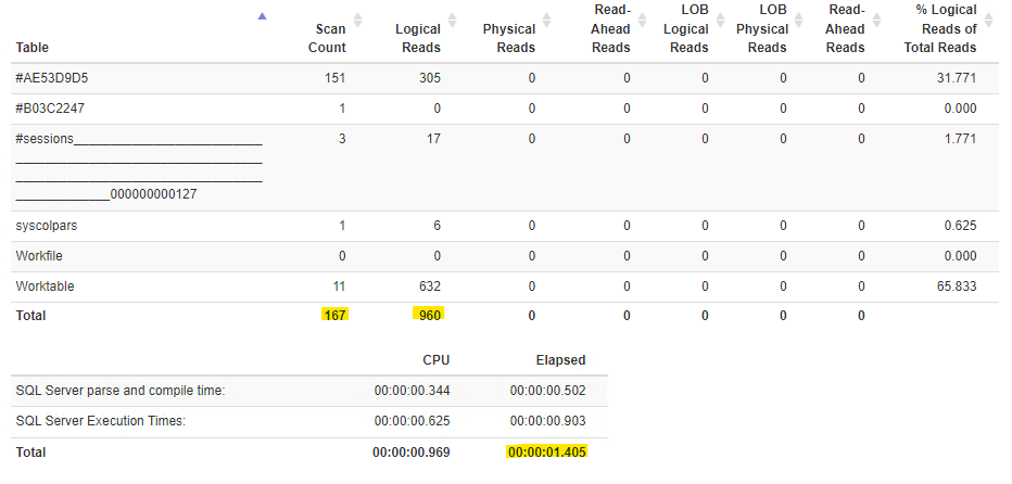
There are three values you’ll want to start with:

• Elapsed – This is the total time that the query took to complete (in seconds).
• Logical Reads – This is the amount of 8k data pages that were read in order to complete this query.
• Scan Count – This is the amount of scans against tables that were performed.

For these three values, lower is better. Before you start tuning make a note of all of these (or a screenshot) so you can see if the changes you make are helping.

Now, Identifying Our Problem

In our next blog post, we will narrow down where exactly our problems lay so that we can get tuning!